Technical note / case report

Pulse dispersion, dielectric mirrors and fluorescence yield: A case report of a two-photon microscope

Peter Rupprecht

Lab of Rainer Friedrich, Friedrich Miescher Institute of Biomedical Research (FMI), Basel, Switzerland

Permanent email: p.t.r.rupprecht+dispersion(at)gmail.com

Key words: dispersion, dielectric mirror, photon yield, two-photon.

Note that this is a limited PDF or print version; animated and interactive figures are disabled. For the full version of this article, please visit https://github.com/PTRRupprecht

Intended audience

Two-photon microscope users who are keen on understanding more about the technical details and especially about what can go wrong with two-photon microscopes.

Summary

This case report describes how a two-photon microscope was found to come with a fluorescence yield that was lower than expected; how the underlying cause was found out in a systematic manner; and how the problem was solved. All approaches and solutions are specific for the microscope under question. However, I hope that this report (1) will inspire other people who are troubleshooting or optimizing their microscopes, (2) will help other people better understand two-photon microscopes and the relevance of technical details.

First, I will describe how the problem (too low photon yield) was identified. Before identification of the problem, the same microscope had been used without obvious hints that there was indeed an issue.

Next, I will describe the possible reasons underlying the problem and how the most likely cause (laser pulse dispersion) could be singled out.

Then, I will explain the tests that allowed to understand which optical component caused the laser pulse dispersion (degraded dielectric mirrors).

Finally, I will describe what was done to circumvent the problem and what else can be learnt from this experience.

Disclaimer and peer review

This case report is not peer-reviewed and will not be submitted for publication in a peer-reviewed journal. If you find any errors or misleading descriptions, or if you think it would be helpful to cite or link to your or someone else's research article or homepage, just send me an (informal) email. I will of course acknowledge your contribution. This report is not a final version and I hope that input from other people will help improve it. Suggestions per email to p.t.r.rupprecht+dispersion(at)gmail.com.

Cite as:

Quantitative comparison of photon yield across setups

In 2018, I was in the lucky situation to use a two-photon point scanning microscope that I had built myself in 2015 [Rupprecht et al., 2016] and therefore knew by heart. It was a microscope based on resonant scanners for video rate 2D imaging and a remote voice coil motor in the spirit of [Botcherby et al., 2008] for fast z-scanning. It was built on top of a galvo/galvo two-photon scanning Sutter scope built in 2007 and used most of the original components, like the MaiTai laser, the pockels cell, mirrors, (scan/tube) lenses and the dichroic. Therefore, there was no reason to assume there was a problem with any of those components.

The point spread function (PSF) of the microscope (ca. 3-4 μm FWHM in z) was okay, given that the beam underfilled the back aperture of the objective. In 2018, I tried to use the microscope for calcium imaging with the calcium-sensing dye OGB-1, which I injected in the (zebrafish) brain area of interest.

However, at some point I noticed that the amount of signal I could get from this setup (from now on called "setup A"; Fig. 1/left) was low when compared to results with a two-photon point scanning Sutter scope ("setup B"; Fig. 1/middle) that was equally built in 2007, used the same laser and an identical objective, with similar laser power below the objective (ca. 20 mW), and with only slightly better PSF (ca. 3 μm FWHM in z).

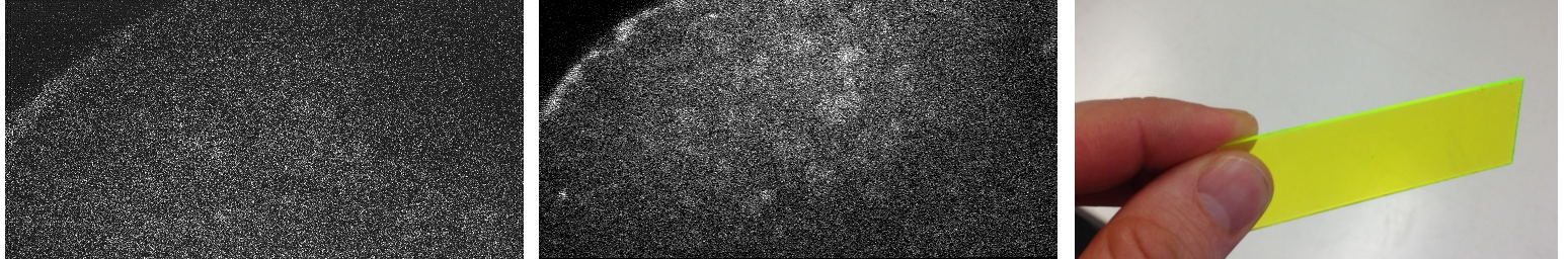
Once determined, the gain factor \(g\) allows to quantify the number of fluorescence photons arriving at the detector using the pixel values of the image. Mean and variance can be taken over the different pixels of the image of a spatially homogeneous sample (Labrigger post), or over the temporal trace of a spatially inhomogeneous but temporally stable fluorescent sample (my previous test). Here, I used the second method with a temporally stable sample, for which I used a cheap fluorescent plastic slide (Fig. 1/right).

As mentioned in the comments on the Labrigger blog post, this quantification can be contaminated by PMT offsets not accounted for (which I measured very carefully) and by multiplicative noise of the PMT cascade. Multiplicative noise adds up to the Poisson noise and therefore creates additional, non-poisson variance in the data, leading to a systematic error of the gain measurement. However, in this special case, where the same PMT type was used both with setup A and setup B at the same PMT gain setting, this systematic error was the same for both setups and could therefore, in a first approximation, be neglected.

The outcome of this quantitative comparison was devastating, indicating that setup A yielded roughly 8x fewer photons compared to setup B at the same conditions! What could be the reason for this huge difference?

The number of detected photons depends both on the number \(N_{photons}\) of photons emitted by excited fluorophors and on the efficiency of the detection path. To test whether this low photon yield was due to the detection path, I simply exchanged the detection pathways of the two systems (including the PMTs, the objective, the dichroic and everything in-between). This was only possible because both systems were quasi-identical Sutter scopes, and the complete detection path could be mounted and unmounted as a whole. However, I observed only a minor change of the photon yield (+15-25%), ruling out a major difference of photon collection efficiencies between the two microscopes.

So what about the number of emitted fluorescence photons? \(N_{photons}\) is influenced by several factors [So et al., 2000]:

with the average power \(P_0\) of the excitation laser, the laser pulse duration \(\tau_p\), the pulse repetition frequency \(f_p\), the numerical aperture NA of the system, the excitaton wavelength \(\lambda_{exc}\), and a couple of factors that are omitted here.

For the two systems, the resolution (reflected by the NA) was roughly the same, as measured by the PSF (see above). Since the very same laser was used for both setups, the pulse repetition rate \(f_p\) was the same for both setups, around 80 MHz, as was the excitation wavelength, \(\lambda_{exc}\), at 920 nm. With the average power \(P_0\) calibrated with a thermal power meter below the objective to be the same for both setups, this left the laser pulse width \(\tau_p\) as the only remaining possible major difference.

The temporal pulse width of a classical Ti:Sa turnkey laser like the MaiTai (Spectra Physics) is just above 100 femtoseconds (fs) when the beam comes out of the laser. Since the product of temporal pulse width and spectral range cannot be below a physical limit (think of the uncertainty principle), these very short femtosecond pulses are actually colored, with a spectral range of ca. 10 nm. The spectral components, however, behave a bit differently depending on the wavelength, leading for example to chromatic aberrations in an imaging system. But also the temporal pulse shape can be affected since red photons travel faster through glass than blue photons. This dependence of the speed of light on the color of light is called dispersion. Many optical components like lenses or objectives therefore can lead to temporal dispersion of the pulse shape. In a typical two-photon point-scanning setup, the 100 fs-pulses coming out from the Ti:Sa laser will usually be dispersed into 300-600 fs-pulses below the objective. Following the equation above, this results in a 3-6-fold reduction of the fluorescence yield, while the average laser power remains unchanged.

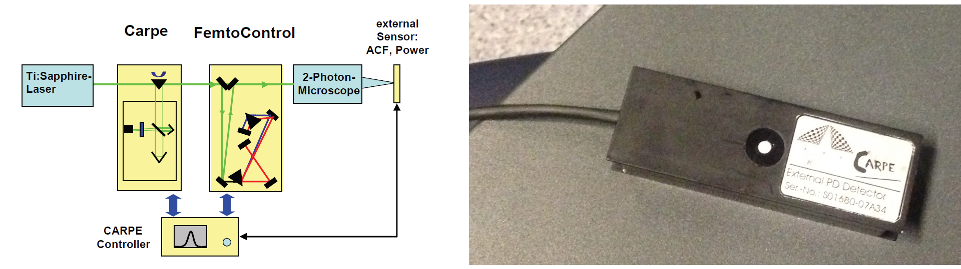
Therefore I measured the pulse width of the laser pulses both right after the laser (or, to be precise, after the pockels cell) and below the objective. Usually, pulse widths are measured using an interferometer and therefore cannot be determined below the objective due to the diverging beam. However, the autocorrelator Carpe (from the company APE) that happened to sit somewhere in a lab cupboard is a device that is designed to perform exactly this task. To describe it very briefly, the Carpe inserts a variable optical delay into the beam path before the microscope, generating two output pulses that are closely spaced in time from one single input pulse. Using the nonlinear dependence of two-photon excitation, a two-photon excitation-based sensor after the microscope (that is, below the objective) can measure the overlap of the two delayed pulses. From the overlap, this device can calculate the pulse width of the original pulse. It is, therefore, a very clever physical implementation of an autocorrelation function (which is a bit broader than the pulse shape).

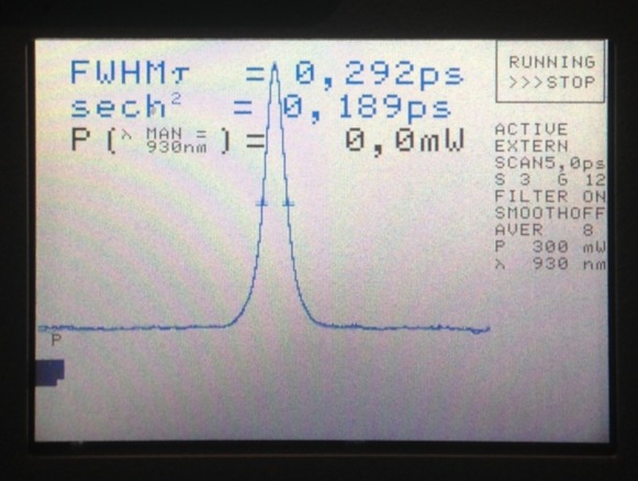
The device therefore does not directly show the pulse shape, but rather the autocorrelation function of the pulse shape. However, it automatically calculates the underlying pulse width. See the legend in Fig. 3 below for a more detailed explanation.

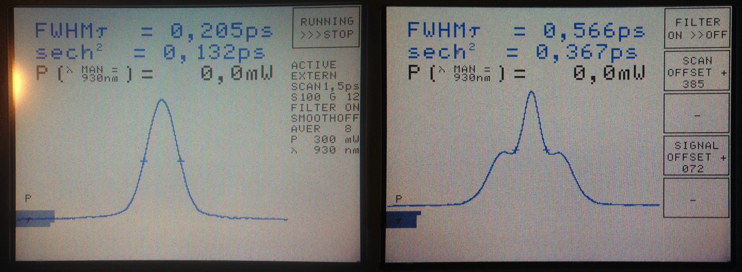
The Carpe autocorrelator is not super-intuitive to work with (for somebody new to this device), but the APE help service turned out to be very supportive, also for in-depth technical discussions. When I first measured the pulse width below the objective, I immediately knew that something was wrong (Fig. 3/right). Not only was the the pulse quite broad in time; in addition, the autocorrelator showed a non-linear distortion of the pulse shape with two heavy shoulders. Obviously, this would be highly detrimental to the fluorescence yield.

The waveform of the autocorrelation function in Fig. 3 suggests that there is not a single pulse, but two pulses. To illustrate this idea more clearly, Fig. 4 shows on the left side a pair of pulses (spaced by few 100 femtoseconds) and on the right side the resulting autocorrelation function. When the two pulses merge to a single one, the trident autocorrelation transforms into a single Gaussian-like shape.

This illustration hopefully makes it easier to understand what a given autocorrelation function means for the underlying temporal pulse shape.

But where did this unusual double-pulse come from?

Possible reasons underlying femtosecond laser pulse distortion

After consultation with the confocal microscopy mailing list and with my PhD supervisor, I had collected a couple of candidate reasons for the strange pulse shape:

1. As mentioned already, the autocorrelation function in Fig. 3 could mean that there are two pulses that arrive shortly one after the other, instead of just one single pulse, as illustrated in Fig. 4. This could be due to an optical element or a coating that creates an internal reflection and therefore a second, delayed pulse.
2. The strange pulse measurement could be due to a measurement error or handling error of the Carpe autocorrelator.
3. According to a very experienced microscopy expert, this "pulse on a pedestal" shape of the autocorrelation functions is a "classic of higher order dispersion caused by large amounts of glass" or other optical elements.
4. Another explanation for the double pulse could be that slightly birefringent material could have been used in the pockels cell or in a polarizing beam splitter. Birefringent material consists of an anisotropic crystal that makes light polarized orthogonal and parallel to the so-called optical axis of this crystal travel faster and slower, respectively. This would result in the laser pulse being split up in two pulses with different polarizations that are delayed one with the respect to the other.

Identification of the underlying problem

1. A double-pulse due to a reflecting interface

As can be seen from the autocorrelation function in Fig. 3 (and as illustrated schematically in Fig. 4), the temporal spacing between the two pulses is around \(\Delta t = 250\) fs. This permits to calculate the approximate physical distance across which the pulse must be reflected:

2. A measurement error

I contacted an engineer of APE, the company that produces the Carpe autocorrelator. He excluded the possibility of a handling error.

3. Dispersion by large amounts of glass

The setup, as described before [Rupprecht et al., 2016], uses a remote scanning unit, resulting in several centimeters of additional glass in the system. This could potentially lead to strong additional dispersion. I therefore removed all lenses (except for scan lens, tube lens and objective) from the microscope. The resulting pulse width was smaller. The shape, however, remained unchanged. Both scan lens, tube lens and objective were the same for the previously mentioned setup B and were therefore unlikely to be the culprit.

4. A double-pulse due to birefringent material

Pulse-splitting by a birefringent material would mean that the resulting double pulse would consist of two pulses of orthogonal polarization. This means that a polarization filter held into the beam path would be able to block out one of the two pulses, depending on the insertion angle.

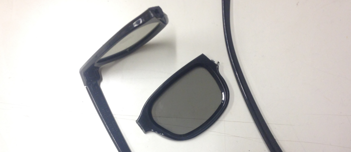
I used goggles leftover from a 3D cinema visit as polarizer. Inserting the polarization glasses into the beam path and rotating the filter reduced the total power of the transmitted light but did not change the temporal pulse shape. This ruled out the possibility that birefringeant material resulted in a double-pulse.

5. Seemingly innocuous optical elements

Therefore something else was the culprit - one of those seemingly innocuous optical elements in the beam path. In total, there were 8 lenses and 3 other glass crystal-based optical elements, and in addition many mirrors of several different kinds. Some of the lenses and mirrors (like the tube lens and the scan lens and a couple of mirrors) could not be easily exchanged. Altogether, quite a daunting task to start with ...

To start with, I removed the entire remote scanning unit (described in [Rupprecht et al., 2016], but for this purpose it's just a big amount of glass), consisting of a polarizing beam splitter, three large-aperture Thorlabs achromats and a small gold mirror. This remote unit was inserted into the system just before the xy-scan unit, i.e., just before the "real" microscope beam path.

Upon removal of this unit, the original pulse shape (black in Fig. 6) was slightly changed - apparently due to linear dispersion - but still deformed in a similar way as before (red in Fig. 6). But this revealed everything I needed to know in order to find the culprit. Let's go into the details.

First, the autocorrelation function measured with the remote scan unit removed (red, dashed lines) was very similar to the original one (black, solid line), but compressed in time. This showed that the nonlinear dispersion responsible for the double-pulse must have happened before this point in the beam path. Why? If the nonlinear dispersion had been generated after this point in the beam path, the lag of the second pulse would have been unaffected by insertion or removal of linearly dispersing glass into the beam path (blue in Fig. 6). From these observations and thought experiments follows a straightforward rule to identify optical components that cause nonlinear dispersion with double pulses: insertion of simple glass with linear dispersion before and after the optical element under question.

Configuration:

Nonlinear dispersion after the removed element No optical element (z-scanning unit) removed Nonlinear dispersion before the removed element Overlay

(Select between the options)

At this point it was clear that the culprit was before the remote scanning unit in the beam path. Yet, there was basically no optical element before the remote scanning unit - except for mirrors.

In retrospect, it is an obvious case: dielectric mirrors. I sorted it out with help from the confocal microscopy mailing list, and all the relevant details have been summarized already by Labrigger in a blog post. In a nutshell, dielectric mirrors consist of many layers of coatings (Fig. 7) that basically act as interference filters, resulting in the reflection of the laser beam.

The dielectric mirrors in this setup were already older than 10 years. In addition, glue had been applied to the rear side of some of the mirrors. Both effects probably caused an irregular spacing of the interference layers of selected locations of some of the mirrors and therefore a highly nonlinear distortion of the temporal pulse shape. This effect was not due to all of the dielectric mirrors, but only 2 or 3 of them, with minor distortive contributions from the other mirrors. To make things a bit more complicated, the incidence angle onto each mirror mattered as well as the incident polarization, and a mirror that worked nicely for one incidence angle produced strong nonlinear dispersion for a different incidence angle.

As any interference effects, the distortions caused by these mirrors also turned out to be strongly wavelength-dependent. As shown below in Fig. 10, the temporal duration and shape of the laser pulse strongly depends on the wavelength (see again the Labrigger blog post for a bit more detail).

However, this strong dependence on the wavelength also allows to check for these pulse shape deformations with no need for a specialized autocorrelator: the deformation of the pulse shape is simply reflected by the fluorescence yield of a stable sample. I used the above-mentioned green plastic slide to record the fluorescence elicited by laser pulses at different wavelengths for both setups:

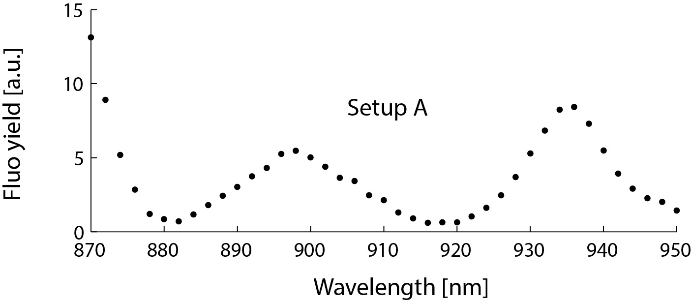
Setup A/B:

Setup B Setup A

(Select between the options)

Of course, the fluorescence yield also depends on the wavelength because both the two-photon excitation cross section of the fluorophor and the output power of the Ti:Sa laser are wavelength-dependent. However, those dependencies are smooth (as for setup B in Fig. 8) and cannot explain the non-monotonous wavelength-dependence observed (setup A in Fig. 8). The result for setup A indicates that the laser pulse is strongly distorted at around 880 nm and 920 nm.

This simple experiment does not inform about the pulse shapes directly. But it is clear from the spectrum in Fig. 8 that "setup A" has an issue related to strong, nonlinear pulse dispersion.

How can we solve the problem?

Solving the problem

To solve the problem, I replaced, as suggested by the confocal microsocopy mailing list, all dielectric mirrors with metal (gold) mirrors. Metal mirrors are coated with very few (protective) interference coatings and are therefore not strongly dispersive. They are actually not more expensive than dielectric mirrors, but are often replaced with dielectric mirrors because the latter offer higher reflectances than metal mirrors.

After replacing everything with gold mirrors, the laser pulse was quite long (FWHM of more than 500 fs), and the fluorescence yield was still by far lower in this setup (setup A) than in the previously mentioned setup B. Therefore, I measured the pulse width in this very impressive setup B, and it turned out to be just above 150 fs below the objective! At this point, I realized that setup B also used some old dielectric mirrors, which, however, did not lead to strange pulse-on-pedestal pulse shapes but instead - by chance - resulted in a highly compressed, optimized, short laser pulse. That was unexpected.

To match the superior performance of setup B, I first inserted a prism compressor (again from the company APE), which is designed to add negative dispersion to the laser pulse, ideally resulting in an optimal, short laser pulse at the sample. However, the alignment turned out to be quite tedious. The additional optical path inside of the prism compressor resulted in a diverging beam path, and I finally did not manage to make it work properly for all wavelengths. Plus, it did not seem to be entirely stable over days, and since I did not have much experience with pulse compressors, I would have taken me probably too long to solve this problem properly. Therefore I chose the quick-and-dirty solution: I switched back to dielectric mirrors.

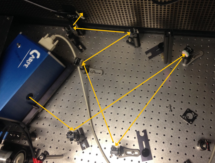
Here is the (close-to-final) result of this random optimization process. The pulse width at 931 nm was around 180 fs (FWHM). Please use the drop-down menu in Fig. 10 (or arrow keys of your keyboard) to go through the wavelength-dependence of the pulse shapes. Due to the nonlinearities contributed by dielectric mirrors, this is not a Gaussian-like curve any more, but it seems to be very close.

Wavelength:

897 nm 898 nm 899 nm 900 nm 901 nm 902 nm 903 nm 904 nm 905 nm 906 nm 907 nm 908 nm 909 nm 910 nm 911 nm 912 nm 913 nm 914 nm 915 nm 916 nm 917 nm 918 nm 919 nm 920 nm 921 nm 922 nm 923 nm 924 nm 925 nm 926 nm 927 nm 928 nm 929 nm 930 nm 931 nm 932 nm 933 nm 934 nm 935 nm 936 nm 937 nm 938 nm 939 nm

(Select between the options)

Conclusion

What I learned from this brief excursion in setup optimization: Dielectric mirrors can dramatically affect the pulse shape of femtosecond lasers (Figs. 3, 6, 10). Dielectric mirrors should be avoided for femtosecond laser pulses in general, especially if they are old; or they should be taken advantage of a) by choosing the best wavelength and/or b) by some sort of random mirror optimization (Fig. 10).

I realized that an autocorrelator can be necessary to understand a microscope based on pulsing lasers. However, recording the wavelength-dependent brightness of a stable object is an alternative source of information about temporal pulse deformations (Fig. 8).

Finally, I have realized that it is possible to work with a setup for years without understanding some of its oddities, and that it can take a lot of time to single down a strange behavior of an existing setup to a specific component or effect. All the more I'm glad that I've returned from this rabbit hole with some lessons learned!

Acknowledgements

For helpful input and discussions, I'd like to thank Craid Brideau, Michael Giacomelli, Zdenek Svindrych, David Chen and Darry McCoy from the confocal microscopy mailing list, Darcy Peterka, Mateusz Ibek from APE Berlin, as well as Tommaso Caudullo and Rainer Friedrich for comments on an earlier version of this report. I'd also like to thank Andrew York for providing an excellent template for scientific publications via Github pages [York, 2017].